GDP Breakdown

GDP components over time and among countries
At the risk of oversimplifying things, the main components of gross domestic product, GDP are personal consumption (C), business investment (I), government spending (G) and net exports (exports - imports). You can read more about GDP and the different approaches in calculating at the Wikipedia GDP page.
The GDP data we will look at is from the United Nations’ National Accounts Main Aggregates Database, which contains estimates of total GDP and its components for all countries from 1970 to today. We will look at how GDP and its components have changed over time, and compare different countries and how much each component contributes to that country’s GDP.
UN_GDP_data  <-  read_excel(here::here("data", "Download-GDPconstant-USD-countries.xls"), # Excel filename
                sheet="Download-GDPconstant-USD-countr", # Sheet name
                skip=2) # Number of rows to skip
#Tidy data
tidy_GDP_data <-UN_GDP_data %>% pivot_longer(cols = 4:51, names_to = "year", values_to = "amount") %>%
#Change names
mutate(IndicatorName=recode(IndicatorName,
`Final consumption expenditure`="consumption_exp",
`Household consumption expenditure (including Non-profit institutions serving households)`="Household expenditure",
`General government final consumption expenditure`="Government expenditure",
`Gross fixed capital formation (including Acquisitions less disposals of valuables)`="gross_fixed_capital",
`Exports of goods and services`="Exports",
`Imports of goods and services`="Imports",
`Gross Domestic Product (GDP)`="GDP",
`Other Activities (ISIC J-P)`="other",
`Agriculture, hunting, forestry, fishing (ISIC A-B)`="agriculture",
`Mining, Manufacturing, Utilities (ISIC C-E)`="mining",
`Wholesale, retail trade, restaurants and hotels (ISIC G-H)`="wholesale",
`Transport, storage and communication (ISIC I)`="transport"),
# Change amount in bn
amount=amount / 1e9) %>%
clean_names()
glimpse(tidy_GDP_data)## Rows: 176,880
## Columns: 5
## $ country_id <dbl> 4, 4, 4, 4, 4, 4, 4, 4, 4, 4, 4, 4, 4, 4, 4, 4, 4, 4, 4~
## $ country <chr> "Afghanistan", "Afghanistan", "Afghanistan", "Afghanist~
## $ indicator_name <chr> "consumption_exp", "consumption_exp", "consumption_exp"~
## $ year <chr> "1970", "1971", "1972", "1973", "1974", "1975", "1976",~
## $ amount <dbl> 5.56, 5.33, 5.20, 5.75, 6.15, 6.32, 6.37, 6.90, 7.09, 6~# Let us compare GDP components for these 3 countries
country_list <- c("United States","India", "Germany")First let us have a look at how the GDP components of United States, India and Germany have fluctuated over years.
#filter the required the indicators
indicator_list <- c("Gross capital formation", "Exports", "Imports", "Government expenditure", "Household expenditure")

#create and filter a temp table
components_table <- tidy_GDP_data %>%
  filter((country %in% country_list), (indicator_name %in% indicator_list))

#reorder the level for the legend
components_table$indicator_name <- factor(components_table$indicator_name, levels = c("Gross capital formation", "Exports", "Imports", "Government expenditure", "Household expenditure"))

#create the graph
components_table %>% ggplot(aes(year, amount, group = indicator_name, color = indicator_name)) +
  geom_line(size=1) +
  scale_x_discrete(breaks=seq(1970,2010,10)) +
  facet_wrap(~country) +
  labs(title = "GDP components over time",
       subtitle = "In constant 2010 USD",
       x = "",
       y = "Billion US$",
       color = "Components of GDP") +

  theme_bw() +

  theme(axis.text.x= element_text(size=7), axis.text.y= element_text(size=7)) +

  NULL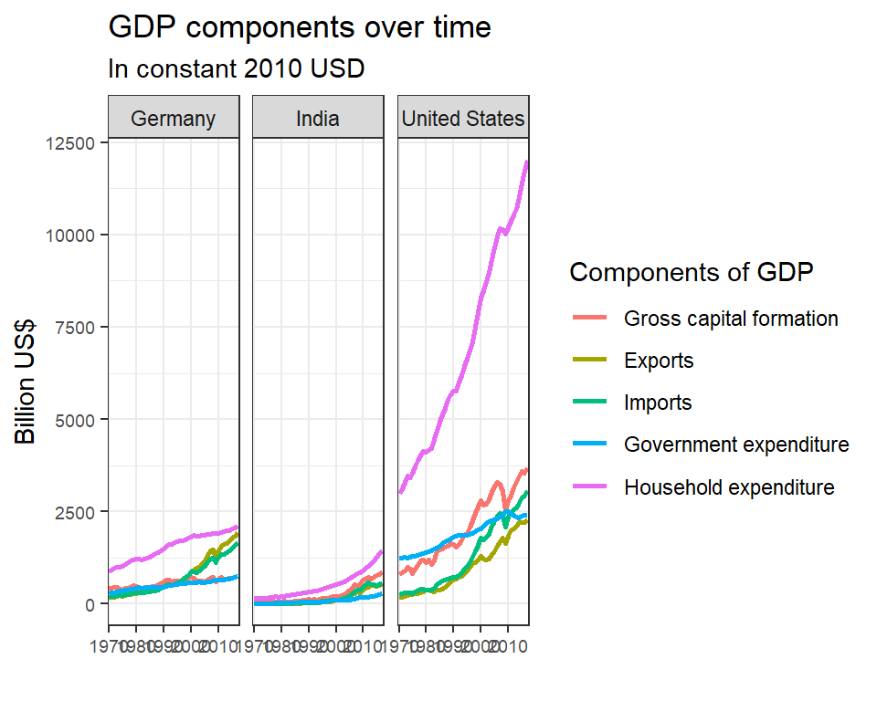
Secondly, recall that GDP is the sum of Household Expenditure (Consumption C), Gross Capital Formation (business investment I), Government Expenditure (G) and Net Exports (exports - imports). Now have a look at the % difference between the calculated GDP and the GDP figure included in the dataframe
indicator_list2 <- c("Gross capital formation", "Exports", "Imports", "Government expenditure", "Household expenditure", "GDP")

gdp_table <- tidy_GDP_data %>%

  #Filter relevant data
  filter(country %in% country_list, indicator_name %in% indicator_list2) %>%

  #Transform to wider format
  pivot_wider(names_from = indicator_name, values_from = amount) %>%

  #Calculate GDP diff
  mutate(Net_exports = Exports - Imports,
         Calculated_gdp = `Gross capital formation` + `Government expenditure` + `Household expenditure` + Net_exports,
         gdp_diff = 100 * ((Calculated_gdp - GDP) / GDP))

gdp_table %>%
  group_by(country) %>%
  summarise(mean_gdp_diff=mean(gdp_diff),
            median_gdp_diff=median(gdp_diff),
            sd_gdp_diff=sd(gdp_diff),
            max_gdp_diff=max(gdp_diff),
            min_gdp_diff=min(gdp_diff))
## # A tibble: 3 x 6
## country mean_gdp_diff median_gdp_diff sd_gdp_diff max_gdp_diff min_gdp_diff
## <chr> <dbl> <dbl> <dbl> <dbl> <dbl>
## 1 Germany 1.14 0.776 1.16 3.56 -0.0411
## 2 India 0.193 -0.198 3.41 7.41 -6.34
## 3 United States 1.27 0.984 1.34 4.55 -0.0522#create the graph
gdp_table %>% ggplot(aes(year, gdp_diff, group = 1)) +
geom_line() +
scale_x_discrete(breaks=seq(1970,2010,10)) +
facet_wrap(~country) +
#Create horizontal line
geom_hline(yintercept=0,
linetype="solid",
color = "red",
size=0.5) +
#Label the graph
labs(title = "% Difference in GDP over time",
x = "Year",
y = "% (calculated over provided GDP)") +
theme_bw() +
theme(axis.text.x= element_text(size=7),
axis.text.y= element_text(size=7)) +
NULL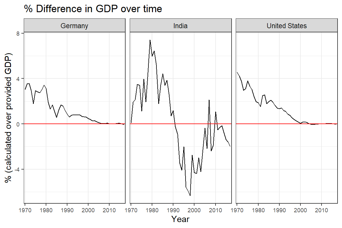
The graphs above show the proportion of the different components that make up GDP by country. For example we can see that India has the highest household expenditure proportion and also comparatively high gross capital formation. For Germany and US, the government expenditure and gross capital formation proportion are closer together. The Net Exports for all countries change along the 0% proportion.
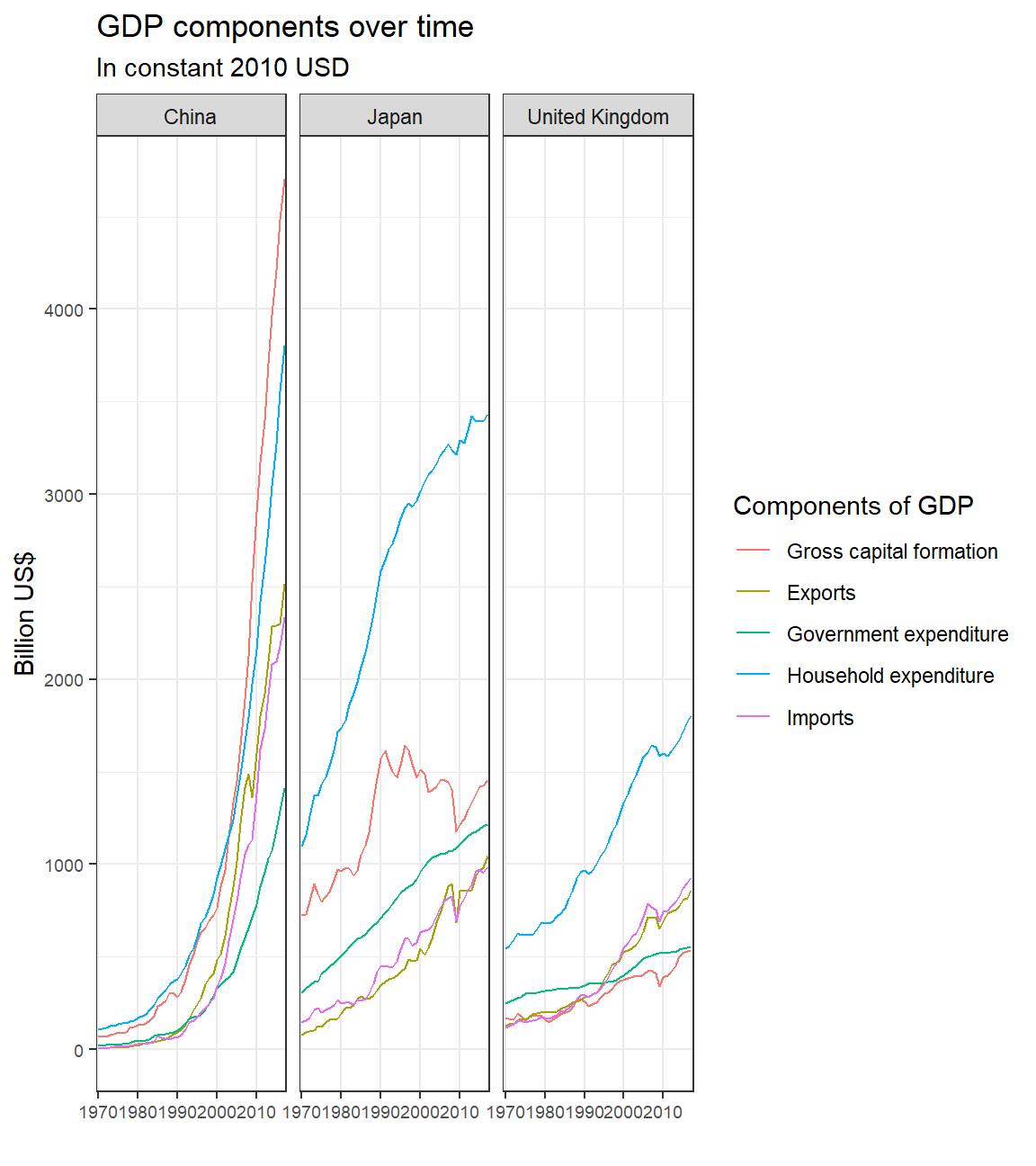
Finally, why not glance at the GDP break down of other three countries?
# Choose these 3 countries
country_list2 <- c("United Kingdom","China", "Japan")

#filter the required the indicators
indicator_list <- c("Gross capital formation", "Exports", "Imports", "Government expenditure", "Household expenditure")

#create and filter a temp table
components_table2 <- tidy_GDP_data %>%
  filter(country %in% country_list2, indicator_name %in% indicator_list)

#reorder the level for the legend
components_table2$indicator_name <- factor(components_table2$indicator_name, levels = c("Gross capital formation", "Exports", "Government expenditure", "Household expenditure", "Imports"))

#create the graph
components_table2 %>% ggplot(aes(year, amount, group = indicator_name, color = indicator_name)) +

  geom_line() +

  scale_x_discrete(breaks=seq(1970,2010,10)) +

  facet_wrap(~country) +

  labs(title = "GDP components over time",
       subtitle = "In constant 2010 USD",
       x = "", y = "Billion US$",
       color = "Components of GDP") +

  theme_bw() +
  theme(axis.text.x= element_text(size=7), axis.text.y= element_text(size=7)) +
  NULL